Wave Function Collapse Algorithm in J

I have heard of the J programming language for a while, but I haven’t written any non-trivial program in J or any array languages. Recently I came across the wave function collapse algorithm that generates sophisticated image without any machine learning model. There are lots of arrays and parallelism in the algorithm, so I decided to implement it to learn a bit of J.

I’ll assume that the reader have read the J primer, just like me when I started this blog. I’ll explain everything in the code in the beginning and gradually reduce the explanation. Also, I’ll intentionally ignore advanced subjects like tacit programming in this post.

The Simplified Algorithm

The original algorithm is too complex to fit in a blog, therefore in this post I’ll implement a special case of the algorithm called ESTM by Robert Heaton. You should read his article and understand the algorithm first.

To make our life as J programmer easier, let me describe the problem and the algorithm with some math notations. ¹

The problem: We have an $m\times n$ input matrix $A$. The elements of $A$ are from a finite set $T=\{0,1,\dots,|T|-1\}$. From $A$ we can obtain some sets of pairs $$S_{up}=\{(p,q)\in T\times T|\exist i\in[0,m),j\in[0,n),A_{ij}=p\wedge A_{i-1\mathrm{mod}\ m,j}=q\},$$ $$S_{down}=\{(p,q)\in T\times T|\exist i\in[0,m),j\in[0,n),A_{ij}=p\wedge A_{i+1\mathrm{mod}\ m,j}=q\},$$ $$S_{left}=\{(p,q)\in T\times T|\exist i\in[0,m),j\in[0,n),A_{ij}=p\wedge A_{i,j-1\mathrm{mod}\ n}=q\},$$ $$S_{right}=\{(p,q)\in T\times T|\exist i\in[0,m),j\in[0,n),A_{ij}=p\wedge A_{i,j+1\mathrm{mod}\ n}=q\},$$

The goal is to create a $p\times q$ output matrix $B$, where for every $i\in[0,m),j\in[0,n)$, $$(B_{ij},B_{i-1\mathrm{mod}\ m,j})\in S_{up},\quad(B_{ij},B_{i+1\mathrm{mod}\ m,j})\in S_{down},$$ $$(B_{ij},B_{i,j-1\mathrm{mod}\ n})\in S_{left},\quad(B_{ij},B_{i,j+1\mathrm{mod}\ n})\in S_{right}. \tag{1}$$

The ESTM algorithm:

1. Create a matrix $B'$ whose elements are subsets of $T$. Initially every element is $T$.
2. Repeat the following until every element of $B'$ only has one element or some of them are empty:
   1. Choose an element $B'_{ij}$ in $B'$. We’ll discuss how to choose it in the following sections.
   2. Choose an element $p\in B'_{ij}$.
   3. The collapse step: set $B'_{ij}=\{p\}$.
   4. The propagation step: set $$B'_{i-1\mathrm{mod}\ m,j}=B'_{i-1\mathrm{mod}\ m,j}\cap N_{up}(p),\quad B'_{i+1\mathrm{mod}\ m,j}=B'_{i+1\mathrm{mod}\ m,j}\cap N_{down}(p),$$ $$B'_{i,j-1\mathrm{mod}\ n}=B'_{i,j-1\mathrm{mod}\ n}\cap N_{left}(p),\quad B'_{i,j+1\mathrm{mod}\ n}=B'_{i,j+1\mathrm{mod}\ n}\cap N_{right}(p),$$ where $$N_{up}(p)=\{q\in T|(p,q)\in S_{up}\},\quad N_{down}(p)=\{q\in T|(p,q)\in S_{down}\}$$ and so on.
3. If every element of $B'$ has only one element (I’ll call such element as a singleton), then we get a valid $B$ by setting the element of $B'_{ij}$ as $B_{ij}$.

Theoretically, the algorithm doesn’t solve the problem because it will generate matrix that violates constraints in (1) under rare circumstances (see appendix A). A more serious issue is that in the propagation step, you have to think in individual elements and their neighbors, not the matrix as a whole, which makes it hard to implement in J. These two problems can be addressed by a slightly different algorithm where the propagation step is applied to all indexes, not just $(i,j)$.

The algorithm to implement:

1. Create a matrix $B^{(0)}$ whose elements are $T$.
2. For $t$ in $0,1,\dots$:
   1. Choose an element $B^{(t)}_{ij}$ in $B^{(t)}$ that is not singleton.
   2. Choose an element $p\in B^{(t)}_{ij}$.
   3. The collapse step: set $B^{(t)}_{ij}=\{p\}$.
   4. The propagation step: create a new matrix $B^{(t+1)}$ where the element at index $(k,l)$ is $$\begin{aligned} B^{(t+1)}_{kl} & =B^{(t)}_{kl}\cap\left(\bigcup_{q\in B^{(t)}_{k-1\mathrm{mod}\ m,l}}N_{down}(q)\right)\cap\left(\bigcup_{q\in B^{(t)}_{k+1\mathrm{mod}\ m,l}}N_{up}(q)\right) \\ &\ \cap\left(\bigcup_{q\in B^{(t)}_{k,l-1\mathrm{mod}\ m}}N_{right}(q)\right)\cap\left(\bigcup_{q\in B^{(t)}_{k,l+1\mathrm{mod}\ m}}N_{left}(q)\right). \\ \end{aligned}\tag{2}$$
   5. If every element of $B^{(t+1)}$ is singleton, then we return a valid $B$ by setting the element of $B^{(t+1)}_{ij}$ as $B_{ij}$. If there is empty set, then we reset $B^{(t+1)}$ to $B^{(0)}$.

Some Intuition

Before we move on to implement the algorithm, I’d like to provide some intuition on these math symbols.

The rules of ESTM can be encoded into a graph. The node set is $T$, and there is an edge from $p\in T$ to $q\in T$ if and only if a tile with type $p$ can be placed next to $q$. $S_{up},S_{down},S_{left},S_{right}$ are the edge set of 4 graphs that corresponds to 4 different directions. The following is an example of the downward graph extracted from a matrix:

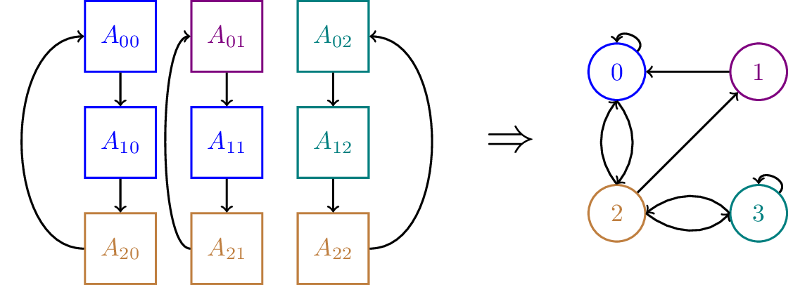
During the propagation step, we look at the neighbors at the chosen index and use the graph to determine which type of tile can be placed there. If the chosen tile has type $p$ and $(p,q)$ is not in $S_{down}$, then the tile below it can not have type $q$. So $N_{down}(p)$ is the set of valid types of tiles that can be place below the tile with type $p$.

From Math to J

It’s fairly easy to write a J program once you have a clean representation of your problem, described in finite sets and matrixes.

The input image can be a text file that contains an integer matrix:

0 0 0 0 0
0 1 1 1 0
0 1 2 1 0
0 1 1 1 0
0 0 0 0 0

We can read the text file and get a matrix in J:

load 'files'
image =: 0 ". freadr 'image.txt'
NB.           freadr      reads a file
NB.      0 ".             convert the string to an array with default value 0

The subset of $T$ is represented by a binary list of $|T|$ elements, where $x$ is in the set iff the $x^{\text{th}}$ element is 1. The matrix $B'$ can be a 3D array.

NB. Get `|T|`
max =: 1 + >./ , image
NB.            ,        Convert the input image to a list
NB.        >./          Gets the maximum value of a list
NB.    1 +              and plus one

NB. Create the matrix `B'` given the shape of output image
NB. The new state is 1 everywhere since every tile can be in every state
new_state =: 3 : '(y, max) $ 1'
NB.                 ,           Concatenate the shape and maximum value
NB.                        $ 1  Create a matrix with 1

We can use edge lists $S_*$ ² to store the graph:

NB. Get the edge list of the input matrix given a direction
NB. Usage: x edge_list direction
edge_list =: 4 : ',/ |: > x; y|.x'
NB.                           |.  Rotate x so the neighboring element moves to
NB.                               the original position
NB.                     >  ;      Creates an array whose first element is x and
NB.                               second element is y|.x
NB.                  |:           Transpose the array. When seen as matrix, its
NB.                               element are the pair (value before rotation,
NB.                               value after rotation)
NB.               ,/              Flatten the matrix

But an adjacency matrix is handy when we need $N_*(p)$ since the $p^{\text{th}}$ row of the matrix is equivalent to $N_*(p)$. We can use matrix unit to construct the adjacency matrix. For example, if the edge set is $\{(1,2),(3,4),(1,3)\}$, then the adjacency matrix is the sum of matrix units $E_{12}+E_{34}+E_{13}$.

NB. Generate a matrix unit E_{ij} given index and shape
NB. Usage: (i,j) unit (shape_x,shape_y)
unit =: 4 : '(i.y) = x +/ . * (1{y), 1'
NB.                                ,  Creates a list (x, 1)
NB.                    +/ . *         Use matrix product to calculate i*x+j
NB.          (i.y)                    Creates a range matrix with shape (x,y).
NB.                                   Its element at (i,j)-th is i*x+y
NB.                =                  This sets the (i,j)-th element as 1 and
NB.                                   others as 0

NB. Get adjacency matrix of a picture given a direction
adj_mat =: 3 : '+./ (image edge_list y) (unit"1) 2 $ max'
NB.                                              2 $ max  Is the size of matrix unit
NB.                 (image edge_list y)                   Creates the edge list which
NB.                                                       is a list of pairs
NB.                                 (unit"1)              Calculate `unit` for each
NB.                                                       pair of the left, generating
NB.                                                       a list of matrix unit
NB.             +./                                       Add all of the matrix units

Entropy

The algorithm says that we need to choose the element that has the smallest entropy, but we haven’t defined what the entropy of a subset of $T$ means.

For a discrete probability distribution $p$ where $\mathrm{Pr}[p=i]=p_i\ (i=0,\cdots,n-1)$, its entropy is $$-\sum_{i=0}^{n-1}p_i\log_2(p_i).$$

Which can be directly translated into a J verb:

NB. Calculate entropy assuming that input is a probability mass function (PDF)
entropy =: 3 : '+/ - y * 2 ^. y'

Let $X$ a subset of $T$, we can define its entropy as the entropy of sampling from $X$, given by Bayes’ rule $$\mathrm{Pr}[x=i|x\in X]\propto\mathrm{Pr}[x\in X|x=i]\mathrm{Pr}[x=i],\quad i=0,\dots,|T|-1.$$

We can have a good guess of $\mathrm{Pr}[x=i]$ by counting the frequency of each element in the input image. We will not normalize the probability until it is used.

NB. Count the presence of a number in given matrix
NB. Usage: matrix count number
count =: 4 : '+/ y = , x'

NB. The PDF of the prior distribution
prior =: image count"_ 0 i. max

The posterior distribution is trivial since $\mathrm{Pr}[x\in X|x=i]$ is equivalent to the $i^{\text{th}}$ element of the list that represent the subset $X$:

NB. The PDF of posterior distribution
posterior =: 3 : '(% +/) y * prior'
NB.                % +/             is a hook. it is equivalent to `y % +/ y`

Now we have a definition of the entropy of the matrix $B'$ that can be transformed into J sentences, but there is a small gap between it and the function we use to determine the element to collapse: the elements that are already collapsed has the lowest entropy, while we need to choose an element that hasn’t been collapsed. The gap can be filled by replacing zeros in the entropy by infinity because an uncollapsed element always have a positive entropy. ³

NB. Replace zero with infinity
replace_zero =: 3 : 'y + _ * 0 =/ y'
NB. This can't be explained here. See appendix B if you are interested.

NB. The matrix we use to choose the element to collapse
entropy_mat =: 3 : 'replace_zero entropy"1 posterior"1 y'

Collapsing an Element

Unlike Numpy, it is hard to write J sentences that returns or uses the index of the element in an array. A more idiomatic way is to use masks (i.e. the array that is 1 at the element you want to choose and 0 everywhere else).

To get the element to collapse in step 2.1, we can use the mask that indicates the minimal values:

min_mask =: 3 : 'y = <./ , y'

This will give us all elements that equal to the minimal value. Let’s take the first element that matches, so only one element will be collapsed at a time:

NB. Keeps the first element that is 1 and drop others
first =: 3 : '(i.$y) = (,y) i. 1'
NB.                    (,y) i. 1  Get the index of the first 1 in `(,y)`

NB. Indicates the element to collapse
collapse_mask =: 3 : 'first min_mask entropy_mat y'

We use roulette wheel selection to choose the element to collapse to in step 2.2.

NB. Roulette wheel selection assuming that input is a PMF
roulette =: 3 : '(((? 2147483647) % 2147483647) < +/\ y) I. 1'
NB.                 ? 2147483647                                Generates a random integer
NB.                               % 2147483647                  Divide them by maximum value
NB.                                               +/\ y         Calculate the running sum of the PMF
NB.                                             <               Create a list that is 1 after some
NB.                                                             random element
NB.                                                      I. 1   Take the index of 1

It’s easier to calculate roulette for the whole $B^{(t)}$ even though we only use the result of one element.

NB. Run `roulette` and return a mask for every element in the matrix
elem_mask =: 3 : '(i.max) ="_ 0 roulette"1 posterior"1 y'

Now we are able to write the J verb that corresponds to step 2.1 in the algorithm:

collapse =: 3 : '(y * -. collapse_mask y) + (elem_mask y) * collapse_mask y'
NB. Here we use the trick introduced in appendix B again

Propagation

In this section we will translate the equation (2) into J sentenses. $\bigcup_{q\in S}N_*(q)$ is just a matrix product given that $N_*(p)$ is just the $p^{\text{th}}$ row of the adjacency matrix:

NB. Get that union of things given a direction
NB. Usage: B' union_of_things direction
unions =: 4 : '((-y) |. x) (+./ . *)"1 _ adj_mat y'
NB.                         +./ . *                  Is the matrix product where `+`
NB.                                                  is replaced by `+.` (union)
NB.              _y                                  The adjacency matrix's direction
NB.                                                  is reversed in equation (2)

Then the propagetion step can be done by taking the intersections of these unions:

NB. Neighbors on the right, left, down, up
neighbors =: 4 2 $ 0 1 0 _1 1 0 _1 0

propagation =: 3 : '*./ y , y unions"_ 1 neighbors'
NB.                           unions"_ 1            Get the unions for all neighbors
NB.                                                 and stack the results
NB.                     y ,                         Add B' to the results
NB.                 *./                             Intersects among the results

Control Flows

The control flow of our algorithm consists of three component:

1. There is a infinite loop
2. If there is an empty set, reset the matrix $B'$
3. If every element of $B'$ is singleton, break the loop

The second part can be placed in the body of the loop:

NB. Reset B' if there is a zero row
valid_or_reset =: 3 : 'y >: *./ , +./"1 y'
NB.                               +./"1   If there is an 1, then it won't be 0
NB.                         *./ ,         Calculate the conjunction among them
NB.                      >:               If rhs is 1, then it returns y,
NB.                                       otherwise returns an array full of 1s

NB. The body of the loop
iter =: 3 : 'valid_or_reset propagation collapse y'

The loop can be written as the power of a verb whose input has the same “type” as output. It stops when the condition is not true:

NB. Continue the loop if there are uncollapsed element
continue =: 3 : '-. *./ , 1 = +/"1 y'
NB.                           +/"1    Count the number of elements in a row
NB.                       1 =         Check whether the count is 1
NB.                (                ) The result of this part stands for
NB.                                   "All elements are collapsed"

NB. The loop
loop =: iter ^: continue ^: _
NB.                         _   Can be an integer to indicate the number of loops

When the algorithm returns, we need to get the output matrix from $B'$:

get_image =: 3 : 'y (I."1) 1'

Putting All Pieces Together

That’s it! A simplified wave function collapse algorithm within a page of J code:

load 'files'
image =: 0 ". freadr 'image.txt'
max =: 1 + >./ , image
new_state =: 3 : '(y, max) $ 1'
edge_list =: 4 : ',/ |: > x; y|.x'
unit =: 4 : '(i.y) = x +/ . * (1{y), 1'
adj_mat =: 3 : '+./ (image edge_list y) (unit"1) 2 $ max'
entropy =: 3 : '+/ - y * 2 ^. y'
count =: 4 : '+/ y = , x'
prior =: image count"_ 0 i. max
posterior =: 3 : '(% +/) y * prior'
replace_zero =: 3 : 'y + _ * 0 =/ y'
entropy_mat =: 3 : 'replace_zero entropy"1 posterior"1 y'
min_mask =: 3 : 'y = <./ , y'
first =: 3 : '(i.$y) = (,y) i. 1'
collapse_mask =: 3 : 'first min_mask entropy_mat y'
roulette =: 3 : '(((? 2147483647) % 2147483647) < +/\ y) I. 1'
elem_mask =: 3 : '(i.max) ="_ 0 roulette"1 posterior"1 y'
collapse =: 3 : '(y * -. collapse_mask y) + (elem_mask y) * collapse_mask y'
unions =: 4 : '((-y) |. x) (+./ . *)"1 _ adj_mat y'
neighbors =: 4 2 $ 0 1 0 _1 1 0 _1 0
propagation =: 3 : '*./ y , y unions"_ 1 neighbors'
valid_or_reset =: 3 : 'y >: *./ , +./"1 y'
iter =: 3 : 'valid_or_reset propagation collapse y'
continue =: 3 : '-. *./ , 1 = +/"1 y'
loop =: iter ^: continue ^: _
get_image =: 3 : 'y (I."1) 1'
(": get_image loop new_state 10 10) fwrites 'output.txt'

I won’t bother writing a GUI for it. A simple vibe-coded webapp is good enough.

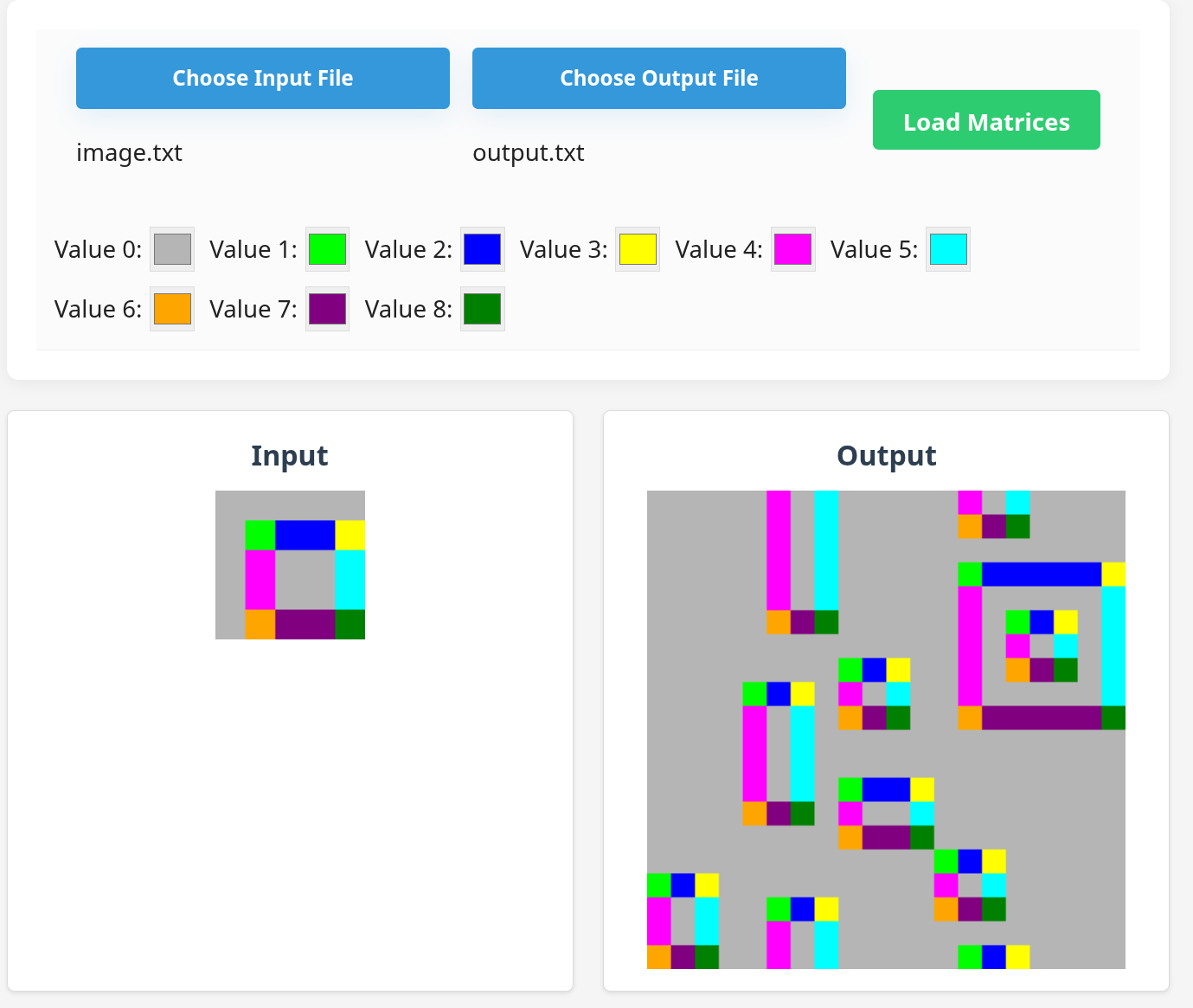
Conclusion

Things I like in J (or array languages in general):

• Programming becomes math. If there is a simple way to describe the problem in matrixes and sets of integers, then writing a J program is trivial.
• You get the benefit of functional programming. Arrays are immutable, you are thinking in functions (or verbs), there are some kinds of type constraint (through array shape and rank) and higher order functions (through combinators).
• It’s not that hard to read. The semantics are simple, and once you understand the basics and know what the words mean, it’s quite readable (I may be wrong because I haven’t learned much about tacit programming).

What’s next: I’ll probably learn some tacit programming and rewrite (golf?) the program, or try other things in J.

Appendix A: The Algorithm is Imperfect

Here’s an example where the original algorithm fails: consider the input matrix $$A=\begin{pmatrix} 3 & 4 & 5 & 6 \\ 1 & 2 & 8 & 7 \\ 3 & 4 & 5 & 6 \\ 11 & 10 & 9 & 7 \\ \end{pmatrix}$$ and a $2\times 4$ output matrix $B$. By collapsing $B'_{10}=\{1\},B'_{00}=\{3\},B'_{01}=\{4\},B'_{02}=\{5\},B'_{03}=\{6\},B'_{13}=\{7\},B'_{12}=\{9\}$, we create a invalid pair $(2,9)$ which doesn’t appear in $S_{right}$.

Our algorithm also fails because the propagation steps is based on stale data. In the example above, it is still possible to generate $(2,9)$ if $$B^{(t)}=\begin{pmatrix} \{3\} & \{4\} & \{5\} & \{6\} \\ \{1\} & \{2,10\} & \{8,9\} & \{7\} \\ \end{pmatrix}.$$

Appendix B: How to Modify Elements in J

We need to write a J verb replace_zero that set the zero elements in an array to infinity (or any number). For example:

1 2 0         1 2 _
0 0 1   -->   _ _ 1
2 3 4         2 3 4

  y       replace_zero y

The example above can be written as from the linear combination of matrix units $$E_{00}+2E_{01}+0\cdot(E_{02}+E_{10}+E_{11})+E_{12}+2E_{21}+3E_{22}+4E_{23}$$ to another linear combination of matrix units $$E_{00}+2E_{01}+\infty\cdot(E_{02}+E_{10}+E_{11})+E_{12}+2E_{21}+3E_{22}+4E_{23}.$$

So a valid replace_zero

1. Finds the matrix units that corresponds to y’s 0
2. Multiply them by infinity
3. Adds them to y

We can directly translate these steps to J:

replace_zero =: 3 : 'y + _ * 0 =/ y'

In general, we can modify the matrix by:

1. Create some masks
2. Decompose the input matrix according to these masks (which is always possible because matrix units are a set of independent basis)
3. Multiply something and add them back

Suppose that we want to set the element of a $3\times 3$ matrix $A$ at index $(0,2),(1,0)$ to 1 and element at index $(1,2)$ to 2. First we can decompose $A$ into these three matrix: $$A_1=A_{02}E_{02}+A_{10}E_{10},\quad A_2=A_{12}E_{12},\quad A_{orig}=A-A_1-A_2.$$

Then the result can be written as $$A_1+2A_2+A_{orig}.$$