Designing 80:20 Rule Languages

EDIT: I made it clearer that the second language is not original.

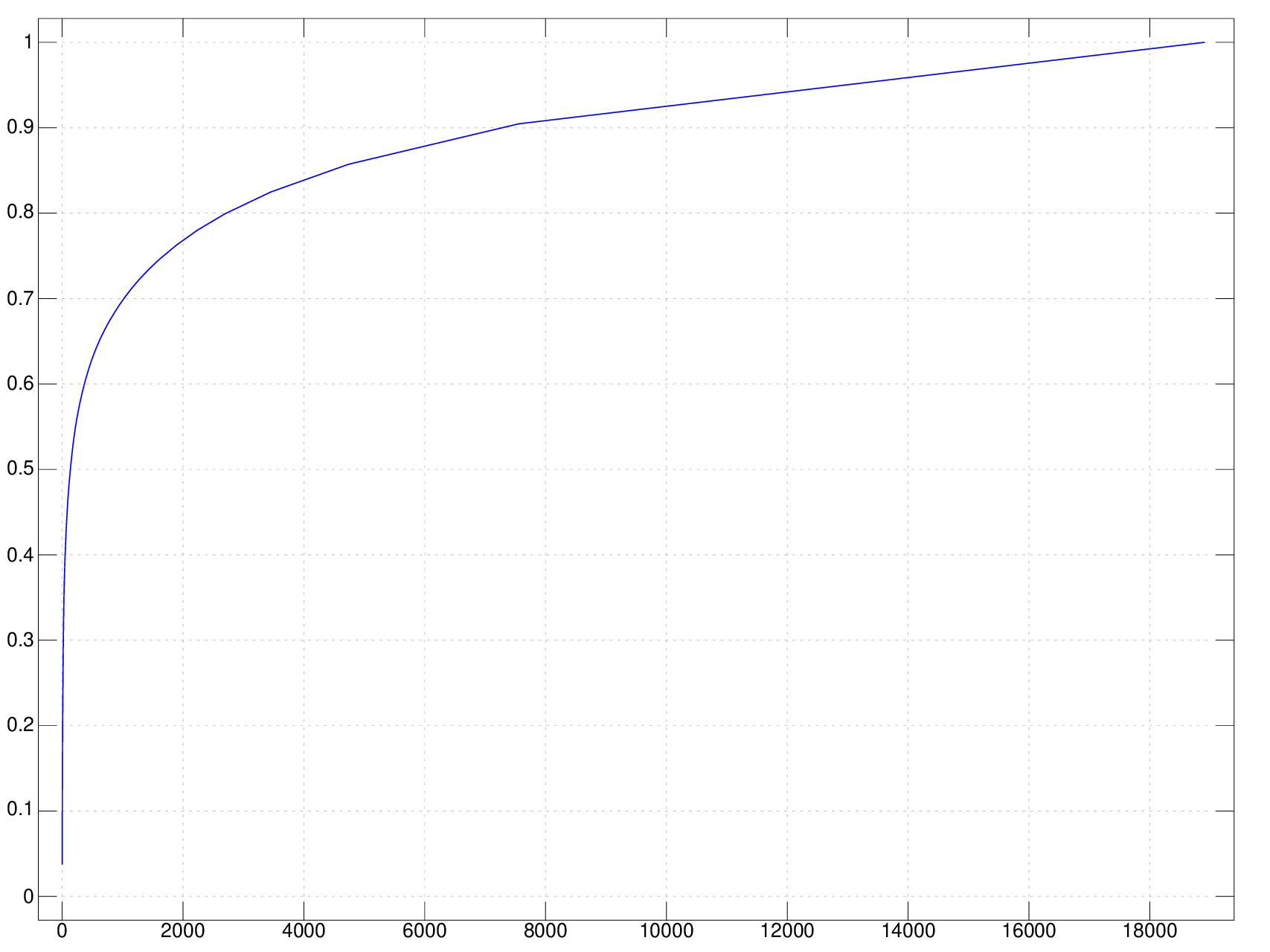
If you calculate a running sum of the sorted frequency of every word in a long book ¹, the result looks like the following curve:

You can try this J program with your favorite book (as long as cutopen supports the language), where count is defined in my previous post: ²

NB. Plot the word count. Your text should only have one newline at the end of
NB. the file, otherwise `freadr` and `cutopen` won't work. J is definitely not
NB. an ideal language for string processing.
plot +/\ (% +/) \:~ (count"_ 0 ~.) cutopen , freadr 'your/book.txt'
NB.                            ~.   finds the unique word
NB.                 (count"_ 0 ~.)  is a monadic hook that gets the word count
NB.             \:~                 sort the word count
NB.      (% +/)                     normalizes it
NB.  +/\                            calculate partial sum

There are 18000 kinds of words used in total, but only 20% of them is used in 80% of the scenarios. This phenomenon is known as the Pareto principle or the 80:20 rule. In this post, we will have some understanding about why this pattern appears, by designing two languages that follows the principle.

A Language With Equal Word Length

The first language is a boring one: every word has the same length.

The syntax of the first language:

1. There is a finite set $\Omega$ called alphabet.
2. A word is an element of $\Omega^n$ where $n$ is a fixed number.
3. Characters in a word are iid samples of some random variable $X$ over $\Omega$.

For example, let $\Omega=\{a,b,c\}$, $n=5$ and the value of $X$ over $a,b,c$ is $0.5,0.4,0.1$ respectively, then a sentence of our language looks like:

aabaa bbbaa aabaa baaba abaca bbbba abaac ...

This can be generated using the following J sentence:

20 5 $ ((roulette"1) 100 3 $ 0.5 0.4 0.1) (({ >)"0) 100 $ < 'abc'

Typical Set and the Asymptotic Equipartition Principle

We will focus on one seemingly arbitrary property of the language: the information content of a word. Let $I$ be the random variable that represents the information content. Given a character $x$, we have $$I(x)=-\log_2\mathrm{Pr}(X=x).$$

Since the characters are iid samples, according to the law of large numbers, for every $\varepsilon>0$: $$\lim_{n\to\infty}\mathrm{Pr}\left(\left|\frac{1}{n}\sum_{i=1}^nI(x_i)-H(X)\right|<\varepsilon\right)=1,\tag{1}$$ where $H(X)=\mathbb{E}[I(X)]$ is the entropy of $X$.

Let $\mathcal{A}=\{x^n\in\Omega^n:|\frac{1}{n}\sum_{i=1}^nI(x_i)-H(X)|<\varepsilon\}$ be the set of words where the average information content is close to the entropy (it’s called the (weak) typical set in information theory). We know from the equation above that you will almost surely get an element of $\mathcal{A}$ when sampling a word, despite that $|\mathcal{A}|$ is relatively small as we will see.

To estimate $|\mathcal{A}|$, let’s consider an element $x^n=(x_1,x_2,\dots,x_n)\in\mathcal{A}$ and try to answer: What’s the probability of getting the word $x^n$?

Here we can make use of the iid assumption again: $$\mathrm{Pr}(X^n=x^n)=\prod_{i=1}^n\mathrm{Pr}(X=x_i)=2^{\sum_{i=1}^n\log_2\mathrm{Pr}(X=x_i)}=2^{-\sum_{i=1}^nI(x_i)}.$$

By definition of $\mathcal{A}$, $$(1-\varepsilon)H(X)<\frac{1}{n}\sum_{i=1}^nI(x_i)<(1+\varepsilon)H(X).$$

Therefore, $$2^{-n(1+\varepsilon)H(X)}<\mathrm{Pr}(X^n=x^n)<2^{-n(1-\varepsilon)H(X)}.$$

We know this is true for every $x^n\in\mathcal{A}$, so the probability of $X^n\in\mathcal{A}$ is lower-bounded: $$2^{-n(1+\varepsilon)H(X)}|\mathcal{A}|<\mathrm{Pr}(X^n\in\mathcal{A}).$$

$\mathrm{Pr}(X^n\in\mathcal{A})$ is a probability, therefore it can’t be greater than 1: $$2^{-n(1+\varepsilon)H(X)}|\mathcal{A}|<\mathrm{Pr}(X^n\in\mathcal{A})\leq1.$$

Then we have this nice upper bound of $|\mathcal{A}|$: $$|\mathcal{A}|<2^{n(1+\varepsilon)H(X)}.$$

The result is a part of the asymptotic equipartition principle in information theory.

Making The Language 80:20

Let go back to our simple language, and find a set of parameters to make it satisfies the 80:20 rule.

The typical set will have less than 20% of the element if $$\frac{2^{n(1+\varepsilon)H(X)}}{|\Omega|^n}<\frac{1}{5}.$$

We can use the probability distribution $(\frac{1}{2},\frac{1}{4},\dots,\frac{1}{2^{|\Omega|-1}},\frac{1}{2^{|\Omega|-1}})$ to ensure that the entropy is always less than 2 for every $\Omega$ that has more than 1 element (see appendix A for the proof).

Setting $m=|\Omega|=8$ and using the result $H(X)<2$, we got the first constraint $$\frac{2^{2n(1+\varepsilon)}}{8^n}<\frac{1}{5}\Rightarrow \varepsilon<1-\frac{1}{2n}\log_2 5.$$

Unfortunately, weak LLN (1) doesn’t tell us how the probability converges as $n\to\infty$, and the simplest way I came up with is to sample a lot of words.

n =: 6
m =: 8
sample =: 100000
NB. We use the constraint above to get a valid epsilon.
eps =: (1 - (2 ^. 5) % 2 * n) - 0.01

NB. The probability distribution
p =: (2 ^ _1 - i. m - 1) , 2 ^ - m - 1

NB. The entropy
e =: entropy p

NB. Sample the words
words =: roulette"1 (sample, n, m) $ p

NB. Take the y-th element of the probability
NB. The `"0` at the end specifies that its rank is 0
take =: 3 : '{: 1 {. y }. p'"0

NB. Calculate their average information content
i =: (+/ % #)"1 - 2 ^. take words
NB.  (+/ % #)   is a fork that calculates the averave

NB. Get the result
(+/ % #) (i < e + eps) *. (i > e - eps)

The probability is about 0.84, so the configuration does give us a language that satisfy the 80:20 rule.

Another Language

I was about to end this post when I read this paper by Conrad and Mitzenmacher. The paper describes a way to generate languages where the length of words are varied and the word count is power-law distribution. Let’s have a look at a simple language described in the paper.

The syntax of the second language:

1. There are only three kinds of characters: $a,b$ and spaces.
2. Each character are iid samples from a probability distribution where $\mathrm{Pr}(a)=p,\mathrm{Pr}(b)=p^2$ and $\mathrm{Pr}(\text{[space]})=1-p-p^2$.
3. A word is a sequence of $a$s and $b$s that are not separated by a space.

Again, let’s generate some sample texts with J:

p =: 0.5
((roulette"1) 100 3 $ p,(p * p),(1 - p * p)) (({ >)"0) 100 $ < 'ab '

The result looks like:

b ab baa ab baa   aa  ba  bb ba aa baaaabbbbabb  ba a aaba abaaaa

Note that there are some extra spaces in the text, but that doesn’t change the probability of word because of the iid assumption.

Zipf’s Law

Our second language is a much richer language: there are an infinitive number of words, and as a result, we can not say that a set of a words’ size is 20% of “the set of all words”. Instead, we will proof that the word frequency in our language (asymptotically) satisfies Zipf’s law.

Zipf’s law: Let the probability of the $i^{\text{th}}$ most frequent word in the language be $f_i$, then $$f_i\propto\frac{1}{(i+\beta)^\alpha}\tag{2}$$ where $\alpha>0$.

If we take the logarithm of $f$, then we have $$\log f=-\alpha\log(i+\beta)+\text{constant},$$

That’s why people usually describe Zipf’s law using straight lines in log-log diagram, like this one: 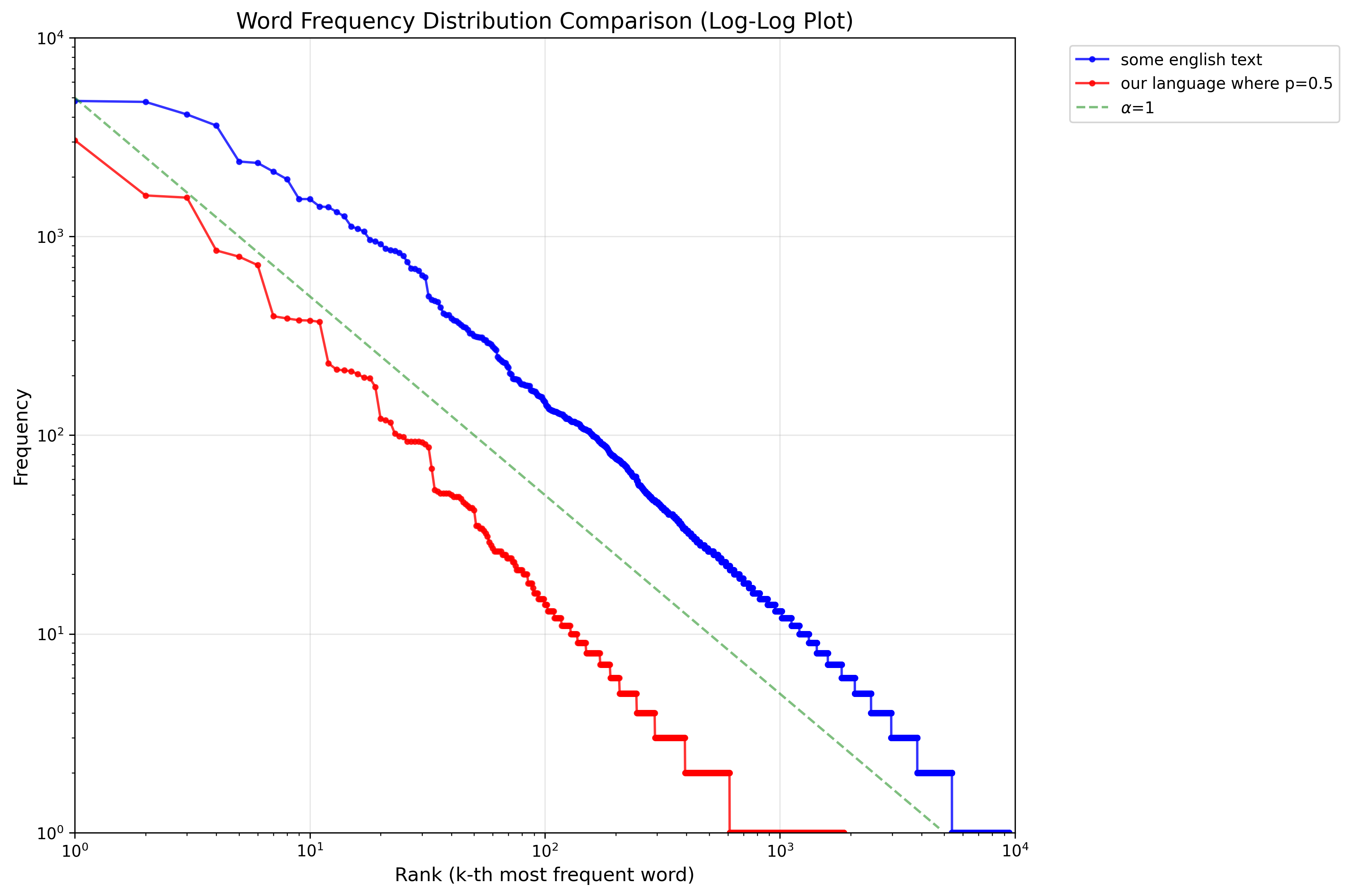(this diagram is plotted using Python and the code is AI-generated, so I won’t paste it here.)

Frequency Ranking and Fibonacci Numbers

To know what the $i^{\text{th}}$ word is, we should sort all the words in our language according to its frequency. The probability of a word with $s$ $a$s and $t$ $b$s (and a space) appearing in a text is $$\mathrm{Pr}(a)^j\mathrm{Pr}(b)^k\mathrm{Pr}(\text{[space]})=p^{s+2t}(1-p-p^2).$$

We can generate the list of words ordered by their frequencies: $$\begin{aligned} S_1=\{a\} & \text{ has probability } p(1-p-p^2), \\ S_2=\{aa,b\} & \text{ has probability } p^2(1-p-p^2), \\ S_3=\{ab,aaa,ba\} & \text{ has probability } p^3(1-p-p^2), \\ S_4=\{aab,bb,aba,aaaa,baa\} & \text{ has probability } p^4(1-p-p^2), \\ & \vdots \\ \end{aligned}$$

Every word can find its place in the list since every word’s probability has the form $p^k(1-p-p^2)$.

You may have noticed that the size of $S_k$ looks like the $(k+1)^{\text{th}}$ Fibonacci number $F_{k+1}$ (and I’m not sorting the words in alphabetical order). Indeed we can proof that $|S_k|=F_{k+1}$, and thus $|S_k|=\frac{\varphi^{k+1}-\psi^{k+1}}{\sqrt{5}}$ (where $\varphi=\frac{1+\sqrt{5}}{2},\psi=\frac{1-\sqrt{5}}{2}$).

The proof. We can proof it by induction.

• $|S_1|=1=F_2$ and $|S_2|=2=F_3$.
• Assume that $|S_{k-2}|$ and $|S_{k-1}|$ are $F_{k-1}$ and $F_k$ respectively. We prove that $$S_k=\{wb|w\in S_{k-2}\}\cup\{wa|w\in S_{k-1}\},$$ where $wa$ means concatenating the word $w$ with $aa$.
  • Because every word in $\{wb|w\in S_{k-2}\}$ and $\{wa|w\in S_{k-1}\}$ has probability $p^k(1-p-p^2)$, therefore $$S_k\supseteq\{wb|w\in S_{k-2}\}\cup\{wa|w\in S_{k-1}\}.$$
  • For a word $w'\in S_k$, if it ends with $a$, then we can strip away the last $a$ to get a word $w$. It has probability $p^{k-1}(1-p-p^2)$, so it will appear in $S_{k-1}$. Similarily, if $w'$ ends with $b$, then stripping away the last $b$ yields a word in $S_{k-2}$. Therefore $$S_k\subseteq\{wb|w\in S_{k-2}\}\cup\{wa|w\in S_{k-1}\}.\ \Box$$

One Last Trick

Finally, we can crack the problem of the frequency $f_i$. If we can write $k$ as an expression of $i$, then its probability is just $p^k$ times a constant.

Here’s the tricky part: we find that writing $k$ as a function of $i$ is harder than the other way, so we instead writing $i$ as a function of $k$ and take its inverse. We have $$\sum_{j=1}^{k-1}|S_j|\leq i\leq\sum_{j=1}^{k}|S_j|,\tag{3}$$ and $$\begin{aligned} \sum_{j=1}^{k}|S_j| & =\sum_{j=1}^{k}\frac{\varphi^{k+1}-\psi^{k+1}}{\sqrt{5}} \\ & =\frac{1}{\sqrt{5}}\left(\sum_{j=1}^{k}\varphi^{k+1}-\sum_{j=1}^{k}\psi^{k+1}\right) \\ & =\frac{1}{\sqrt{5}}\left(\frac{\varphi^{k+1}-1}{\varphi-1}-\frac{\psi^{k+1}-1}{\psi-1}\right). \\ \end{aligned}$$

Because $|\psi|<1$, when $k$ is large, $\psi^{k+1}$ is close to 0, and the equation (3) becomes $$C_1\varphi^{k}+C_2-\varepsilon\leq i\leq C_1\varphi^{k+1}+C_2+\varepsilon,$$ where $C_1,C_2$ are constant that we don’t care about, and $\varepsilon$ is a relatively small value (in terms of $k$).

Then we have $$\begin{aligned} & \frac{1}{C_1}\log_\varphi(i-C_2-\varepsilon)-1\leq k\leq\frac{1}{C_1}\log_\varphi(i-C_2+\varepsilon), \\ \Rightarrow\ & p^{\frac{1}{C_1}\log_\varphi(i-C_2-\varepsilon)-1}\leq p^k\leq p^{\frac{1}{C_1}\log_\varphi(i-C_2+\varepsilon)}, \\ \Rightarrow\ & \frac{1}{p}(i-C_2-\varepsilon)^{\frac{1}{C_1}\log_\varphi p}\leq p^k\leq(i-C_2+\varepsilon)^{\frac{1}{C_1}\log_\varphi p}. \end{aligned}$$

Note that $C_1>0$ and $\log_\varphi p<0$, therefore the equation holds when $i$ is sufficiently large.

Conclusion

These two languages can’t fully explain the 80:20 pattern in natural languages, because we made an assumption that characters are iid, while characters in natural languages are not independent. For example, If you are asked to fill the blanks in t_ese t_ree words with one kind of character, you will choose h rather than e despite that the probability of e in English is higher than that of h. A better probabilistic model requires deep understanding of linguistics and better mathematical tools.

The concept of typical set and AEP are derived from chapter 4 of MacKay’s ITILA textbook. The first language is also influenced by its examples. Fixed-length words are widely used in computing, and typical set provides a way to compress them. In fact, the famous Shannon’s source coding theorem can be described as: we can compress our language without losing too much information, by only encoding the words in the typical set.

I have already mentioned that the second language is paraphrased from this paper by Conrad and Mitzenmacher. The paper proofs that the power-law distribution applies to languages with any probability distribution on a finite set of characters, not just $(p,p^2)$ on two characters.

Appendix: Why the Entropy is Always Less than 2

We want to prove that: for every $m>2$, $$H_m=-\frac{1}{2^{m-1}}\log_2\frac{1}{2^{m-1}}-\sum_{i=1}^{m-1}\frac{1}{2^i}\log_2\frac{1}{2^i}<2.$$

We can simplify $H_m$ to $$H_m=\frac{m-1}{2^{m-1}}+\sum_{i=1}^{m-1}\frac{i}{2^i}.$$

The proof consists of two parts:

1. $H_m$ increases monotonically,
2. $\lim_{n\to\infty}H_m=2$.

The first part is simple: $$H_{m+1}-H_{m}=\frac{m}{2^m}-\frac{m-1}{2^{m-1}}+\frac{m}{2^m}=\frac{1}{2^{m-1}}>0.$$

For the second part, consider the series (we can get this by taking the derivative of the series $\sum_{i=0}^\infty x^n$) $$\sum_{n=1}^\infty nx^{n-1}=\frac{1}{(1-x)^2}\quad(-1<x<1).$$

Let $x=\frac{1}{2}$, then we have $$\sum_{n=1}^\infty\frac{n}{2^{n-1}}=4\Rightarrow\sum_{n=1}^\infty\frac{n}{2^n}=2.$$

Therefore $$\lim_{m\to\infty}H_m=\lim_{m\to\infty}\frac{m-1}{2^{m-1}}+\lim_{m\to\infty}\sum_{i=1}^{m-1}\frac{i}{2^i}=2.$$